WP1 Biogeochemical model calibration and evaluation
Task 1.2 Revisit of Iron sources in PISCES model (Icebergs and sea-ice)
Iron is a critical limiting micronutrient in the Southern Ocean, but its chemistry is complex; moreover, it has multiples sources, not all of which have been accounted for in ocean biogeochemical models. To better evaluate how “new” sources of iron to the Southern Ocean, previously unaccounted for in ocean models, in terms of how they affect ocean biogeochemistry, two model configurations were set up, one to assess effects of iron delivery from icebergs and the other to assess that from sea ice. Both relied on the eORCA1 (nominal 1° grid) configuration of the NEMO-LIM-PISCES ocean model. To assess effects of iron delivery from icebergs, we prescribed that the water flux from Southern Ocean icebergs (Merino et al., 2016, a monthly climatology) had a dissolved iron concentration of 4.5 nmol L-1, as estimated from Raiswell et al. (2008). This iceberg iron source modified the simulated surface distribution of dissolved iron (Fig. 1) resulting in substantial changes in the spatiotemporal evolution of surface chlorophyll concentration (Fig. 2).
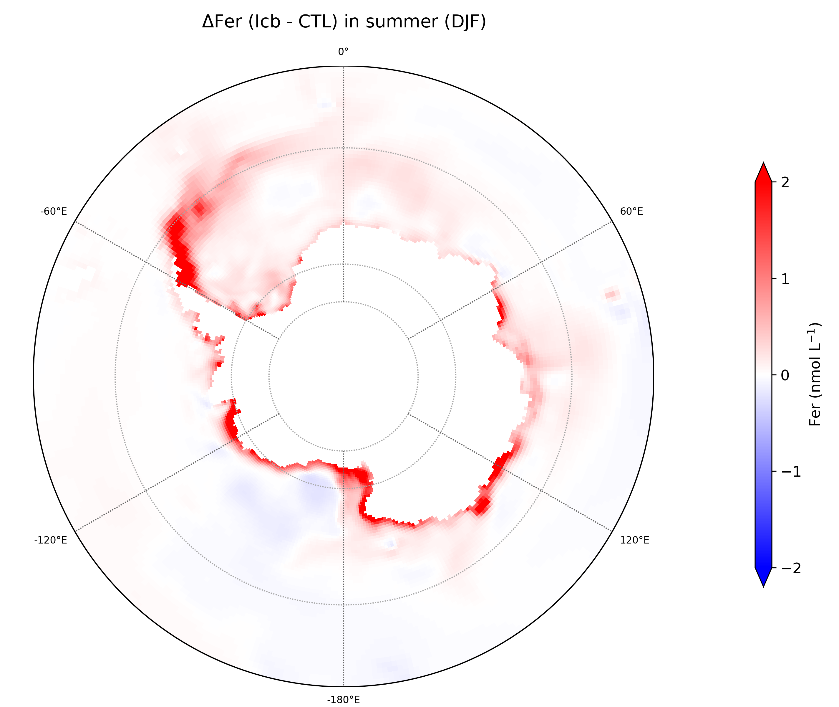
Figure 1. Difference in spatial distribution of the surface dissolved iron concentration in summer between the “iceberg” experiment (ICB, with iceberg iron source) and the control experiment (CTL, , no iceberg iron source).
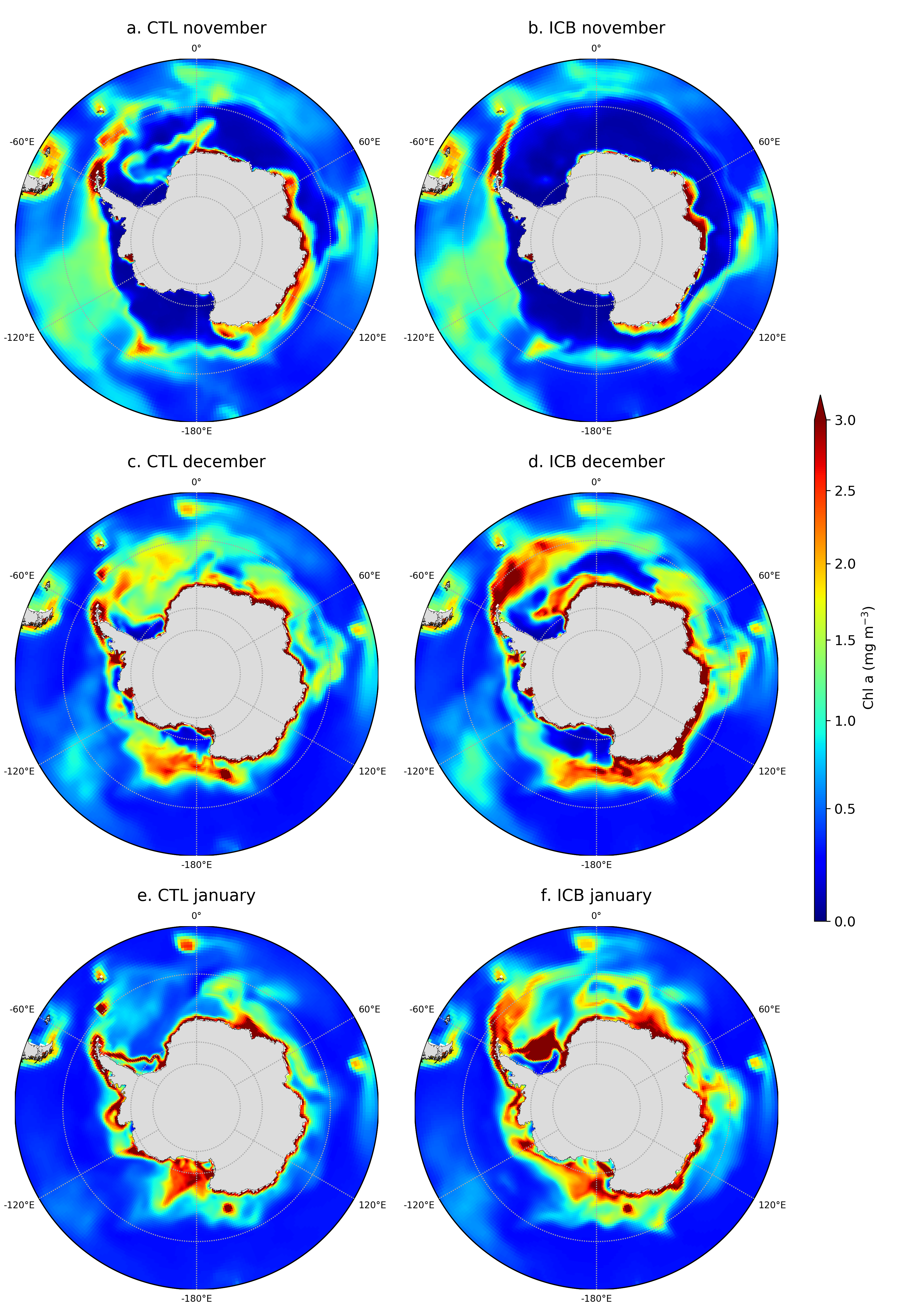
Figure 2. Surface chlorophyll concentration in (left) the CTL experiment (no iceberg iron delivery) and in (right) the ICB experiment (with iceberg iron delivery) in November, December, and January in the Southern Ocean, south of 55°S.
A second configuration was set up to better represent the sea-ice iron source to the Southern Ocean via the sea-ice model (LIM) to the PISCES model. That is, in LIM we added a new variable, the iron content in sea-ice for each ice category. This variable is computed as a function of the iron availability in surface seawater in PISCES based on 2 different seawater-to-sea-ice flux formulations: (1) maintaining a constant maximal iron concentration of 10 nmol L-1 in sea-ice, and (2) a constant iron flux from surface seawater to sea ice of 1x10⁻⁶ nmol s-1. The latter is expected to better represent of what it is observed in the ocean (Lannuzel et al., 2016). Figure 3 shows a comparison in winter and summer of the spatial distribution of surface iron concentration in the PISCES model in the experiment with no iron in sea-ice (Fe CTL) and the experiment with a maximal iron concentration in sea-ice (Fe CST) and their difference.
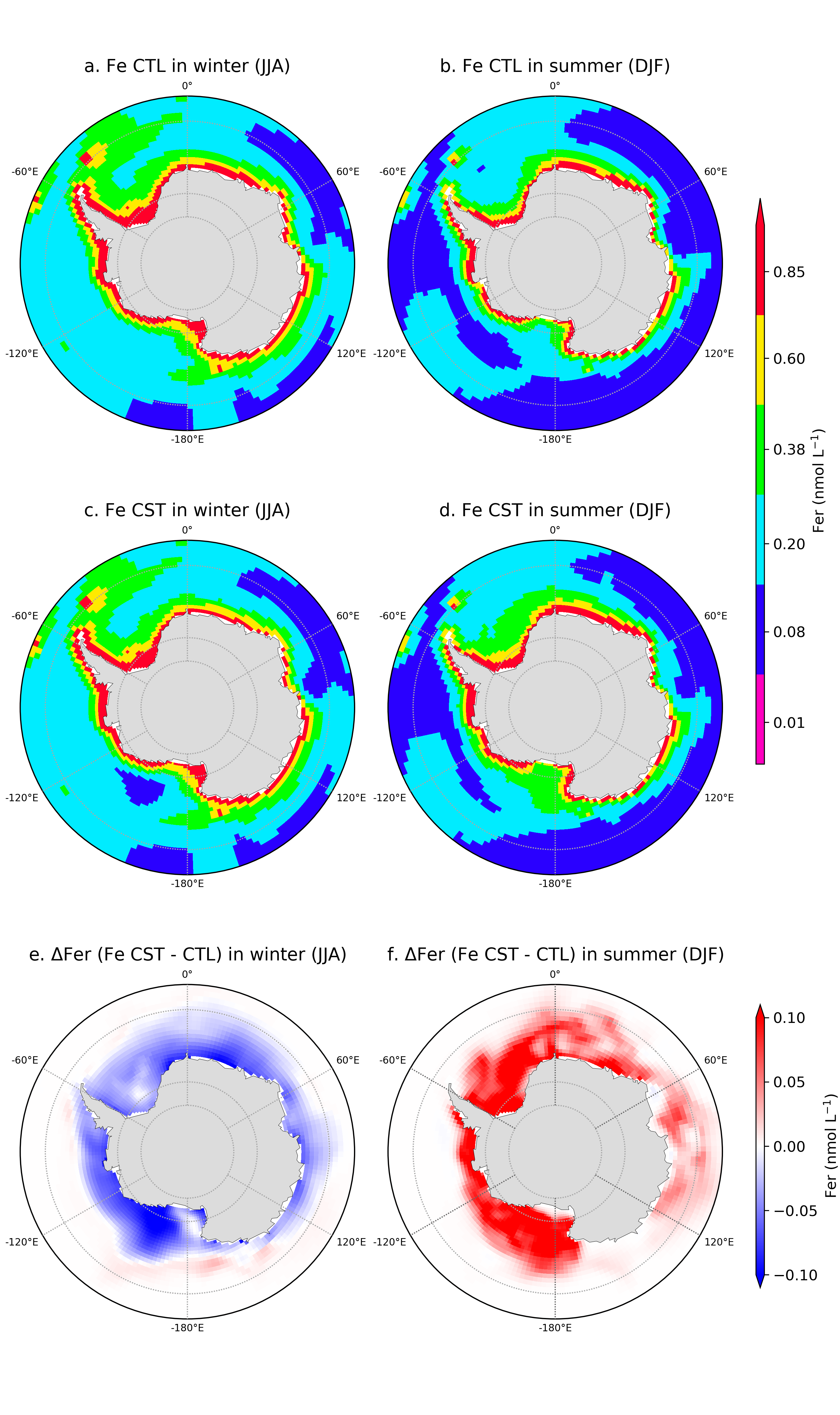
Figure 3. The iron concentration in surface seawater in the Southern Ocean, south of 55°S for (a, b) the control experiment (Fe CTL, no iron in sea-ice), (c,d) the Fe CST experiment, and (e,f) difference (Fe CST minus FeCTL) in austral winter (June, July, August) and summer (December, January, February).
Concurrently during SOBUMS, related work on improving simulated ocean biogeochemistry in the context of the iron-limited Southern Ocean has led to an article that was published in J. Geophys. Res. Oceans in 2018. This study focused on the role of iron in diatoms and how that affects the biological pump and the seasonal cycle of pCO2 (Person, Aumont, & Lévy, 2018)). To cope with iron limitation in the Southern Ocean diatoms, a dominant phytoplankton group in that region, have been shown in cultures to have developed an original adaptation strategy to maintain efficient growth rates despite very low cellular iron quotas, even in low light conditions. With the NEMO-PISCES model, we explored the consequences of this physiological adaptation for the biological pump and the seasonal variability of both surface chlorophyll and surface pCO2. In the PISCES model, we implemented a low intracellular Fe:C requirement in Southern Ocean diatoms. Relative to the control experiment (CTL), that new formulation (PHYSIO) exhibits a 10% increase in the relative contribution of diatoms to total Southern Ocean primary production, which strengthens the biological pump and enhances the biological contribution to the seasonal evolution of pCO2 relative to the thermodynamic component. When compared to the observations, the simulated seasonal cycle of both surface chlorophyll and surface pCO2 in the Polar Zone (PZ) are markedly improved in PHYSIO vs. CTL . This improvement is noteworthy given that virtually all ocean models, whether forced or coupled, have had major difficulties to simulate the seasonal cycle of pCO2 in the Southern Ocean, the region that takes up most of the ocean's anthropogenic carbon and heat.
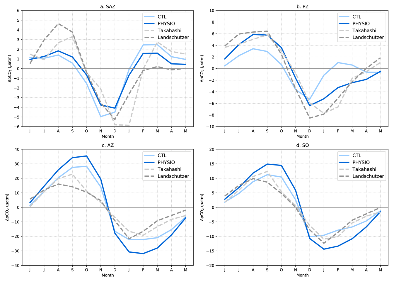
Figure 4. Seasonal cycles of the anomalies of ∆pCO2 (pCO2oc – pCO2atm) from observations, (Landschützer [dashed line, dark grey] and Takahashi data set [dashed line, light grey]), the CTL experiment (light blue), and the PHYSIO experiment (dark blue) averaged over (a) the Sub-Antarctic Zone (SAZ), (b) the Polar Zone (PZ), (c) the Antarctic Zone (AZ), and (d) the entire Southern Ocean (SO) south of the subtropical front.
Reference:
Lannuzel, D., Vancoppenolle, M., van der Merwe, P., de Jong, J., Meiners, K. M., Grotti, M., … Schoemann, V. (2016). Iron in sea ice: Review and new insights. Elementa: Science of the Anthropocene, 4, 000130. https://doi.org/10.12952/journal.elementa.000130
Merino, N., Le Sommer, J., Durand, G., Jourdain, N. C., Madec, G., Mathiot, P., & Tournadre, J. (2016). Antarctic icebergs melt over the Southern Ocean: Climatology and impact on sea ice. Ocean Modelling, 104, 99–110. https://doi.org/10.1016/j.ocemod.2016.05.001
Person, R., Aumont, O. & Lévy, M. (2018). The Biological Pump and Seasonal Variability of pCO2 in the Southern Ocean: Exploring the Role of Diatom Adaptation to Low Iron. J. Geophys. Res. Oceans. https://doi.org/10.1029/2018JC013775
Raiswell, R., Benning, L. G., Tranter, M., & Tulaczyk, S. (2008). Bioavailable iron in the Southern Ocean: the significance of the iceberg conveyor belt. Geochemical Transactions, 9(1), 7. https://doi.org/10.1186/1467-4866-9-7